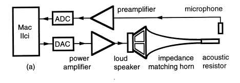
Figure 1. Schematic diagrams indicating (a) the acoustic impedance spectrometer, and its connection to (b) the reference cylindrical pipe and (c) the embouchure hole of the flute.
J R Smith, N Henrich & J Wolfe
School of Physics
The University of New South Wales
Sydney 2052 Australia
In this paper we report precise and rapid measurements of the impedance of a flute at the embouchure hole. Impedance measurements offer several advantages, providing not only information on the resonance frequencies, but also their relative magnitudes and sharpness. For any given fingering, the Q of the various resonances and their deviations from an exact harmonic series is important in determining stability of intonation - approximately what many musicians call being well 'centred'. They are also important in the ease of 'speaking' or 'starting' of notes, and in transitions between notes.
Impedance measurements on the flute impose several technical problems. Although the impedance curves for instruments with reed and lip-reed instruments have been measured for many years, e.g. [2,3], such instruments sound at frequencies determined by their impedance maxima. The air column of the flute is excited by an air-jet at an embouchure hole which is open to the external air, so the flute sounds at frequencies near the impedance minima. Impedance measurements should thus cover a very wide dynamic range, often exceeding 60 dB.
For the player and maker, all of the notes are virtually equally important so all of the standard fingerings must be studied. Professional players use alternate fingerings in some circumstances, and the contemporary repertoire requires special fingerings for microtones, multiphonics and different timbres. Measurements should be rapid for this reason, and also if they are to be used in diagnosis of problems and successive improvements in flutes. In this study we use a 'real time' technique developed for research into the acoustical impedance of the vocal tract [4,5]. We use a frequency spacing of 1 Hz and determine the detailed shape of the impedance, and thus the resonances, to ±0.5 Hz.
Figure 1. Schematic diagrams
indicating (a) the acoustic impedance
spectrometer, and its connection to (b)
the reference cylindrical pipe and (c)
the embouchure hole of the flute.
Calibration
In the calibration procedure, an electrical waveform with a
power spectrum denoted by VREF(f) is synthesized and
converted by the loudspeaker, horn and high acoustic resistance
into an acoustic current uREF(f), which is coupled to a
reference load ZREF(f). The acoustic pressure is measured via
the microphone and the pressure spectrum pREF(f) calculated.
A new waveform with Fourier components proportional to
VREF(f)/pREF(f) is then synthesized. This produces a
spectrum that is flat (i.e. frequency independent to ±0.1 dB
rms) when pREF(f) is measured.
The system was calibrated using a resistive load as ZREF. This was a semi-infinite pipe - (in practice a 42 m stainless-steel pipe with an internal diameter of 7.8 mm, i.e. slightly smaller than the embouchure hole - see Figure 1b). For measurements when the frequency spacing exceeds 4 Hz, the calibration can be performed before the echo returns and so the 42 m tube is effectively infinite. For 1 Hz resolution, a 1 s waveform was required. Fortunately, the attenuation in a tube of this diameter is approx. 0.11 per metre [7] at 200 Hz, so the echo returned with a loss of 80 dB and thus made negligible change in the amplitude measured in the calibration signal. The -18 dB level on our plots of Z(f) corresponds to 2.2 MRayl.
Coupling the flute to the spectrometer
The acoustic current source with a flat spectrum uREF(f) was
then coupled to the embouchure hole of the flute using the
measurement head shown in figure 1c. It was designed to
measure the impedance at the embouchure hole when it is
loaded with an impedance approximately equal to the radiation
impedance of the hole with the player's lips and face acting as a
baffle.
We report measurements for frequencies below 3 kHz and thus with wavelengths exceeding 100 mm. This is rather larger than the dimensions of the measurement head and so a plane wave approximation should be valid. The radiation impedance of a baffled pipe of radius a is approximately equal to that of an ideal tube with a length L = 0.85a. The radiation impedance ZE at the embouchure hole could thus be approximated by
ZE = jwrL/SE = 0.48 jwr/(SE0.5)
where SE denotes the effective area of the embouchure hole, w = 2pi.f and r denotes the density of air.In the playing position, the embouchure hole is partially occluded by the lower lip leaving open a fraction g. Furthermore the face of the player will act as a baffle over a fraction (1-h) of the solid angle available for radiation. ZE is thus increased to ZE = 0.48 jwr/h(gSo)0.5 when the flute is in the playing position and where So denotes the unencumbered area of the embouchure hole.
The short measurement tube of length LT that couples the spectrometer to the embouchure hole has an area ST and its impedance is ZT = jwrLT/ST. ZT will thus equal ZE when LT = 0.48ST/h(gSo)0.5 where So is the actual area of the embouchure hole (approx. 80 mm2). The factor g will vary because any one player will occlude the hole by different amounts for different notes, and h will also vary among players because of the shape of their faces. Consequently the term hg1/2 cannot be known precisely, although we suspect it is less than 0.5. For our adaptor we chose a tube with ST less than So because this makes positioning less critical, and also because it improves the plane wave approximation. The selected tube had a diameter of 7.8 mm and consequently LT = 7 mm if we assume h = g = 0.5.
Impedance measurements on the flute
The measured pressure spectrum p(f) will be given by
p(f) = uREF(f) ZFLUTE(f) = pREF(f)ZREF(f) ZFLUTE(f) = constant . ZFLUTE(f)/ZREF(f)
where the constant is known from the calibration procedure described above. The semi-infinite pipe should exhibit a frequency-independent acoustic resistance. Consequently the measured pressure spectrum p(f) immediately yields ZFLUTE(f).The time taken to acquire the data to calculate each plot of Z(f) was only 1 second, although calculation of the Fourier components from the data sampled at 44.1 kHz took considerably longer. To allow replication by others, all measurements were made on a basic production line flute (Pearl PF-661, closed hole, C foot) rather than the finer instruments of our industry collaborator. Measurements were made in dry air with T = 19.5±0.5 C.
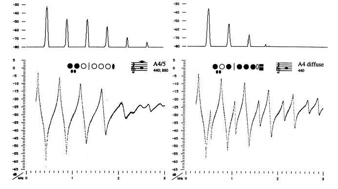
Figure 2 The lower plots show the impedance spectra of a flute measured at the embouchure hole with (a) the conventional fingering for A4/5 and (b) an alternate fingering for A4. Each plot is a set of points representing measurements at 2801 different frequencies. The upper continuous lines show the measured pressure spectrum from the sound of another flute played with the same fingering.
Figure 2a shows Z(f) for the standard fingering used to play both A4 (440 Hz) and A5. The first four tone holes are closed and all others are open. The inset shows the fingering (some keys close two tone holes). Below about 1.9 kHz, the curve may be compared with that for a simple cylinder of length chosen to sound A4. Above that frequency, the open tone holes downstream produce subtle effects. Even 'venting' (opening or closing the seventh tone hole downstream) makes a clearly observable difference to Z(f), though it has little effect on the note produced. The flute is played with the embouchure hole at least partly open, and so the minima of Z(f) correspond to playing frequencies. For the fingering A4/5 shown the flute can be made to play notes near each of at least the first four of these minimum frequencies by blowing harder in turn, and adjusting the embouchure. (A clarinet, on the other hand, is played with a mouthpiece and reed that more closely approximates a closed end. The clarinet too is cylindrical, to first order, and it plays at maxima of impedance. A clarinet mouthpiece driving this load would be expected to sound the frequencies of the maxima - i.e. approximately the odd harmonics of a fundamental roughly half that of the flute.) A detailed analysis of the flute has been published by Coltman [8] among others.
The plots in Figure 2a show an asymmetry of the peaks in Z(f) for the flute which is not seen in Z(f) for a simple pipe. This may be qualitatively explained as follows: One difference between a flute and a simple cylinder is that the embouchure hole is displaced from one end, and that it is smaller than the diameter of the flute. Further, it is in general partly occluded by the player's lower lip, as discussed above. The reduction in diameter is expected to have relatively little effect on the impedance maxima, where the flow is low and pressure high. It is expected to have a rather larger effect on the impedance minima, where flow is high and pressure is low. Thus the minima are flattened with respect to the maxima.
Figure 2b shows Z(f) for another fingering for A4 (A4/II from [9]). 3.2 This fingering produces a diffuse, dark timbre, some broadband jet noise and a limited dynamic range. It overblows to rather brighter notes at approximately A5, E6 and A#6.
Impedance for different constructions
Can measurements of Z(f) explain superiorities in actual
performance? Here we give a simple example using the same
flute with no geometric changes.
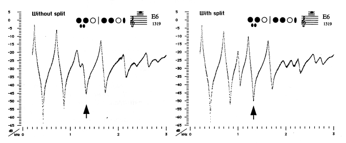
Figure 3 The impedance spectra Z(f) for the note E6 on a flute with and without the 'split E' mechanism. The vertical arrows indicate the frequency at which this note sounds.
The two spectra in figure 3 show the effect of a 'split E' mechanism. This fingering (and the spectra) can be considered in (at least) two different ways. If one regards it as E4 with the third finger of the left hand raised, then it produces the fourth harmonic of this note. In a flute with the mechanism, raising that finger opens one tone hole, which forms a pressure node about 1/4 of the way along the tube. Without the mechanism, two adjacent tone holes are opened. This has a similar effect, but in this case the E6 is less reliable at pianissimo (notice the shallower, broader minimum indicated by the arrow) and difficult to play cleanly under a slur from A4 or A5. One may also think of this fingering as a perturbation of that for A4/5 (Fig 2a) with some holes closed downstream. Notice how Z(f) of the split E version is more dissimilar to Z(f) for A4/5, which explains the increased ease of the slur A4/5-E6.
The impedance for 'multiphonics'
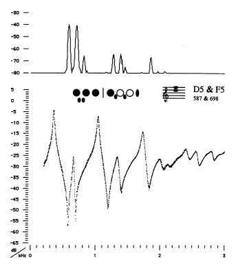
Figure 4 The impedance spectrum (lower curve) and sound pressure spectrum (upper curve) for a fingering that produces 'multiphonics' - it plays D5 and F5 simultaneously. The peaks in the sound spectrum have a common factor of approx 120 Hz, which is presumably the periodicity of the air jet.
Impedance for the standard fingerings
The impedance spectra for the standard
fingerings between C4 and F#7,
and those for selected non-standard and multiphonic
fingerings are available at our website -
/music/flute/.
The support of the Australian Research Council is gratefully acknowledged. We would also like to thank John Coltmann, Neville Fletcher, John Tann and Mark O'Connor (Lehner Flutes Aust and The Woodwind Group) for their assistance.
 Flute Acoustics -
Measurements
Flute Acoustics -
Measurements
Flute Acoustics
Musical Acoustics Group
School of Physics, UNSW